Advanced aero for ORC racing. Cut-sheet inputs. Explainable Edge Map.
Layer 2 consumes richer sail geometry (width stations / trapezoid stacks) and optional aero overrides from the sail schema. The result is an Edge Map that is not just colored squares, but a defensible engineering artifact: click any cell and trace the delta through coefficients, CE/CLR, depower, and provenance.
Partner lofts and naval architects access these capabilities through Expert Mode.
Seven steps from ORC baseline to performance delta
Every computation in SailEdge™ by SailrScience follows the same cascade. Your ORC certificate
enters at Step 1 as the certified baseline. Each subsequent step builds on the
previous, and the output is a complete performance picture — with every number
traceable back to the ORC data that anchored it.
For a behavior-level walkthrough of this cascade, see The Physics.
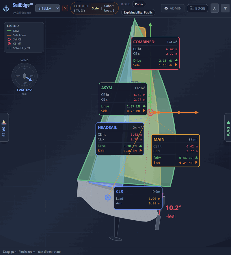
Sitella (Cape 31) at TWA 125° — three sails with per-sail CE cards, drive and side forces, combined CE, CLR with lead and arm. Explainability: Public.
1
Stability / Righting Moment
The baseline that holds the boat up
Your ORC certificate provides RM@1° — the certified stability anchor.
The engine generates a full righting moment curve from 0° to 60° at 1°
increments, using a GZ curve family keyed to that single value. Every step
downstream builds on this curve.
2
Base Aerodynamic Coefficients
What the sails do in the wind
For each sail configuration, the engine computes lift (CL), drag (CD), and
side-force (CY) coefficients along with Center of Effort position
(CEx, CEht). Upwind and downwind regimes use separate
coefficient models — the aerodynamics above and below beam reach are
fundamentally different. Apparent wind derives from the wind triangle.
3
Downwind Regime Blend
The transition between two worlds
Between 90° and 120° TWA, the engine blends upwind and downwind
coefficients using a smooth λ function — C¹ continuous
(smoothstep), no artificial crossover points. CL and CD are blended in
coefficient space; derived force components follow. CE shifts are applied
smoothly across the same λ window.
4
CE Calibration Loops
Tuning the model against what the boat actually does
The engine runs iterative calibration loops that adjust CE position to match
observed behavior. Two independent targets: helm load (rudder angle within
expected bounds for the point of sail) and heel angle (compared against ORC
heel data when available). CE adjustments are bounded to physically plausible
ranges. Every adjustment emits provenance metadata — what moved, how far,
and why.
5
Heel Equilibrium Solve
Where the forces balance
The engine solves for the heel angle where aerodynamic heeling moment equals
hydrostatic righting moment from Step 1. Deterministic bisection on
[0°, 50°] — no convergence tolerance issues. The equilibrium heel
is the physically correct answer for that sail configuration and wind condition,
measured as a delta from ORC baseline.
6
Depower Trigger + Transforms
What happens when the boat is overpowered
When equilibrium heel exceeds the heel limit, the engine computes a depower
factor: the ratio of available righting moment to demanded heeling moment.
Five independent transform channels — lift reduction, drag increase,
CE height drop, CE aft shift, and effective area reduction. The delta between
full-power and depowered performance is what you see in the data.
7
Final Forces + Performance Outputs
The numbers you use to make decisions
Drive force, side force, final heel, rudder angle, boat speed, and VMG —
all computed for this specific sail configuration at this specific wind
condition. Each output carries provenance: RM source (ORC vs. estimate),
CE calibration adjustments applied, depower status, and an overall stability
confidence flag. Every number is a measured delta from your ORC-certified
baseline.
Sail Geometry + Aero Fidelity
Planform distribution matters (and now the model can see it).
ORC racing sails often differ in performance even when the headline numbers look similar (same area, same rig).
Layer 2 captures the distribution of area and chord along the span using stacked stations (a trapezoid stack).
That distribution drives centroid/CE placement, effective aspect ratio, induced drag, and ultimately the Edge Map delta.
Trapezoid slice (two stations)
Ai = ½ (ci + ci+1) · Δzx̄i = (ci2 + cici+1 + ci+12) / (3(ci + ci+1))z̄i = zi + Δz · (ci + 2ci+1) / (3(ci + ci+1))
Here c is chord length at each station and Δz is the vertical separation.
This captures squaretops/blockheads because chord can increase aloft.
Area-weighted centroid over a stack
C = Σ(Ai · ci) / Σ(Ai)
In implementation the model can compute each slice centroid either analytically (as above) or by decomposing the slice into triangles and area-weighting
— both produce the same result when done consistently.
Centroid vs Center of Effort (CE) — why they’re not the same
The centroid is purely geometric. The CE is where the aerodynamic force effectively acts.
For simple sails, centroid is a strong proxy. For modern shapes (deep roach, forward-loaded Code/Asym), CE can be forward of the geometric centroid.
Layer 2 therefore treats CE as: geometric planform + bounded, sail-type-aware transforms + regime-aware blending.
The transforms are designed to stay physically plausible and to preserve explainability.
Schema-driven aero overrides (optional)
When a sail includes an aero block in the sail schema, the model can consume bounded overrides and efficiency modifiers
(e.g., effective aspect ratio and regime-specific multipliers). This allows two sails with the same area to produce different Edge Map outcomes
based on planform quality and loft intent, without requiring a full rewrite of the physics engine.
Sail Interaction
Blanketing is real. The model accounts for it.
The mainsail blankets the headsail on deep angles. The engine measures it.
Each headsail sample point is tested for mainsail occlusion. Blocked points
receive a wake-attenuation weight:
Wake attenuation
w(d) = exp(−(d / d0)β)
Effective unblocked fraction
Feff = Σ(ai · w(di)) / Atotal
Headsail CL and CD are corrected by Feff. The correction ramps between
95° and 150° AWA — outside that window, Feff = 1.0.
Sheeting angle influences the slot geometry between main and headsail and is
carried as a plan input per sail. Corrected forces feed directly into the
combined CE weighting.
Model Boundaries
Hull speed is a boundary. We enforce it.
A displacement hull can’t outrun its bow wave. The engine enforces a
hull-speed fence — a displacement-derived upper bound beyond which
predicted deltas lose physical meaning.
Hull-speed limit
Vhull = 1.34 × √LWL
When computed boat speed approaches this limit, the engine clamps performance
predictions rather than extrapolating into planing territory the hull can’t
reach. Deltas near the fence carry a diagnostic flag. The result: green cells in
the Edge Map appear only where the boat can actually use the speed.
The Output
Baseline vs. edge. Regime by regime.
The Edge Map computes a speed delta for every cell in the TWA × TWS matrix.
Each cell is a controlled comparison: baseline configuration vs. edge configuration,
computed at identical wind conditions within the same regime.
Regimes are independent. A sail that gains 0.3 kt reaching doesn’t inherit
credit from a different regime. Apples to apples, cell by cell.
Every delta carries its upstream signals: centroid CE, occlusion correction,
hull-speed fence, depower status. Tap any cell and trace the number back
through the pipeline.
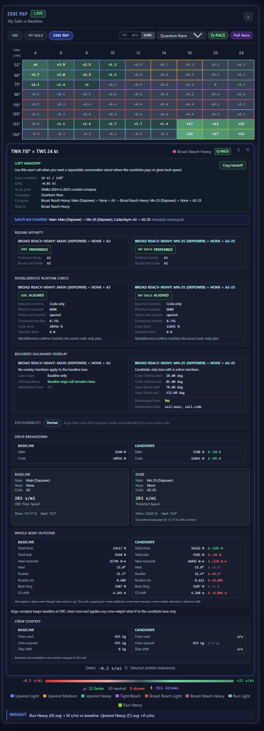
Sitella Edge Map cell detail — baseline vs. edge comparison with runtime context, force attribution, whole-boat outcome, and confidence disclosure.
Data Architecture
Stateless. Deterministic. Inspectable.
The engine is stateless — the View sends boat, sails, and polars with every
request. The physics engine retains nothing between computations. Same inputs produce the same outputs,
every time. Partner environments maintain tuning profiles and model parameters in the
application layer — the physics computation itself remains stateless.
Every computed point carries provenance: RM source (ORC certificate vs. estimate),
CE calibration adjustments applied, depower status, and a confidence flag. When the
Edge Map shows +0.3 kt, you can see whether that number is anchored to a full ORC
stability curve or an estimated one — and whether the engine had to adjust CE
to make the helm behave.
The delta is still real. The provenance tells you how much to trust it.
Validation
Tested against real boats.
The model has been validated against 20+ ORC-certified boats, including a Cape 31 that
won its class at Key West Race Week. Validation checks include: boat speed vs ORC target
polars, force-balance behavior under depower, CE position vs helm angle, and heel
convergence at stability limits.
Where the model diverges from an ORC target, provenance tags show exactly where the
divergence originates — estimated RM, CE calibration offset, or aero coefficient
bounds. The gap is visible, not hidden.
Full Reference
Inspectable outputs and model health signals.
Every computed point produces outputs, constants, and diagnostic signals. On the public site we describe what they mean without exposing internal API key names.
Stability Outputs
Output
Units
Description
Equilibrium heel
deg
Equilibrium heel before clamping — the raw physics answer
Final heel
deg
Final heel after depower clamp
Depower factor
0–1
Ratio of available RM to demanded heeling moment
Certified RM@1°
kg·m
ORC-certified righting moment (baseline anchor)
Righting moment at equilibrium heel
N·m
Righting moment at equilibrium heel
Righting moment at heel limit
N·m
Righting moment at heel limit (depower reference)
Heeling arm
m
Effective moment arm: CE height + CLR depth
Heeling moment (raw)
N·m
Heeling moment before depower
Heeling moment (post-depower)
N·m
Heeling moment after depower application
Rudder / Helm Outputs
Output
Units
Description
Rudder angle (clamped)
deg
Rudder angle after clamping
Rudder angle (unclamped)
deg
Raw rudder angle before safety clamp
Helm load index
kN
Yaw-moment-to-arm ratio — helm load index
Yaw moment
kN·m
Net yaw moment from CE–CLR offset
CE–CLR longitudinal separation
m
Fore–aft distance between CE and CLR
Rudder force needed
N
Force required to balance yaw moment
Dynamic pressure (water)
Pa
Hydrodynamic pressure at boat speed
Force + Performance Outputs
Output
Units
Description
Driving force
kN
Net forward driving force
Side force
kN
Net lateral (heeling) force
Boat speed
kt
Predicted boat speed (with depower coupling)
VMG
kt
Velocity made good toward wind or mark
% of ORC baseline polar
%
Performance as percentage of ORC baseline polar
Combined CE fore–aft
m
Combined CE fore–aft position (from mast datum)
Combined CE height
m
Combined CE height above deck
Combined CE lateral offset
m
Combined CE lateral offset under heel
Physics Constants
Constant
Value
Notes
ρair
1.225 kg/m³
Standard sea-level air density
ρwater
1025 kg/m³
Seawater density
g
9.81 m/s²
Gravitational acceleration
kts → m/s
0.5144
Knots to meters per second
Tuning Parameters (Categories)
Layer 2 uses a small set of bounded tuning parameters to keep CE/CLR behavior physically plausible across the boat library.
We do not publish parameter names or values publicly. Partner-private coefficient sets and overrides live in Layer 3 under NDA.
Category
What it governs
Why it matters
CE geometry
CE height, fore–aft position, heel-induced shifts
Sets heeling arm and helm balance; drives heel and yaw moment
CLR geometry + dynamics
CLR position, depth, speed effects
Sets CE–CLR separation and lift response; affects helm load
Rudder + helm limits
Rudder lift slope and angle limits
Converts yaw moment into a feasible rudder angle and flags constraints
Depower thresholds
Heel limits and depower floors
Controls when the model transitions from full power to depowered behavior
Coupling + convergence
Iteration count and damping
Ensures stable, deterministic performance solutions across conditions
Diagnostic Signals
Every computed point carries a diagnostic bitfield. When the engine encounters
edge cases or physically unusual conditions, it flags them rather than hiding them.
Public pages describe the signal meaning (not the internal bit numbers).
A
Above baseline polar
Computed speed exceeds the ORC baseline polar — unusual but possible with favorable sail delta
B
Negative drive
Net drive force is negative — drag exceeds thrust in this configuration
C
Apparent wind near zero
Apparent wind speed is near zero — edge case where the wind triangle collapses
D
Heel exceeds limit (raw)
Raw equilibrium heel exceeds defined limit — depower will activate
E
Rudder at limit
Rudder angle hits a safety clamp — the boat needs more helm than available
F
Non-finite numeric value
Computation produced a non-finite result — flagged for investigation
G
Heel clamped at limit
Final heel is clamped at the limit — depower is active, performance reduced
H
Depower active
Depower transforms are applied — the delta includes sail-loading reduction